Quick start guide for NRP 3.2

Introduction

The NRP is designed to be an easy-to-use, intuitive interface for in silico brain simulation experiments. An experiment typically includes a virtual agent or “body” performing a specific task using a dedicated brain model in a simulated environment. While brain models can be implemented through a variety of simulators, the simulated environment is always provided by the simulator called Gazebo.

Our community of users mostly includes roboticists, computational neuroscientists, and engineers working on applications of neuromorphic computing. However, anyone with a working knowledge of Python can easily learn how to use our platform.

This quick start guide shows you how to set up and run a simple experiment - connecting a robot’s control command to two oscillating neurons so that the robot will start waving its arm - by using a network of spiking neurons created with the simulator called NEST.

Step 1. Access the NRP

You can access the NRP either online with your EBRAINS account or locally, after installation on your machine (see this page for differencies). Regardless of how you log in to the NRP, you will have access to the same GUI (displayed below in Fig. 1, the “Experiment overview”).

First-time users must accept EBRAINS Terms and Conditions before accessing our software.

1. Go to https://neurorobotics.net/access-the-nrp.html.

2. Choose between online access or local installation.

3. Create an EBRAINS account at https://ebrains.eu/register.

4. Choose between versions 3.05 and 3.2.

5. Follow the link and login with your username and password.

Congratulations! You can now start using the NRP via its “Experiment overview” interface.

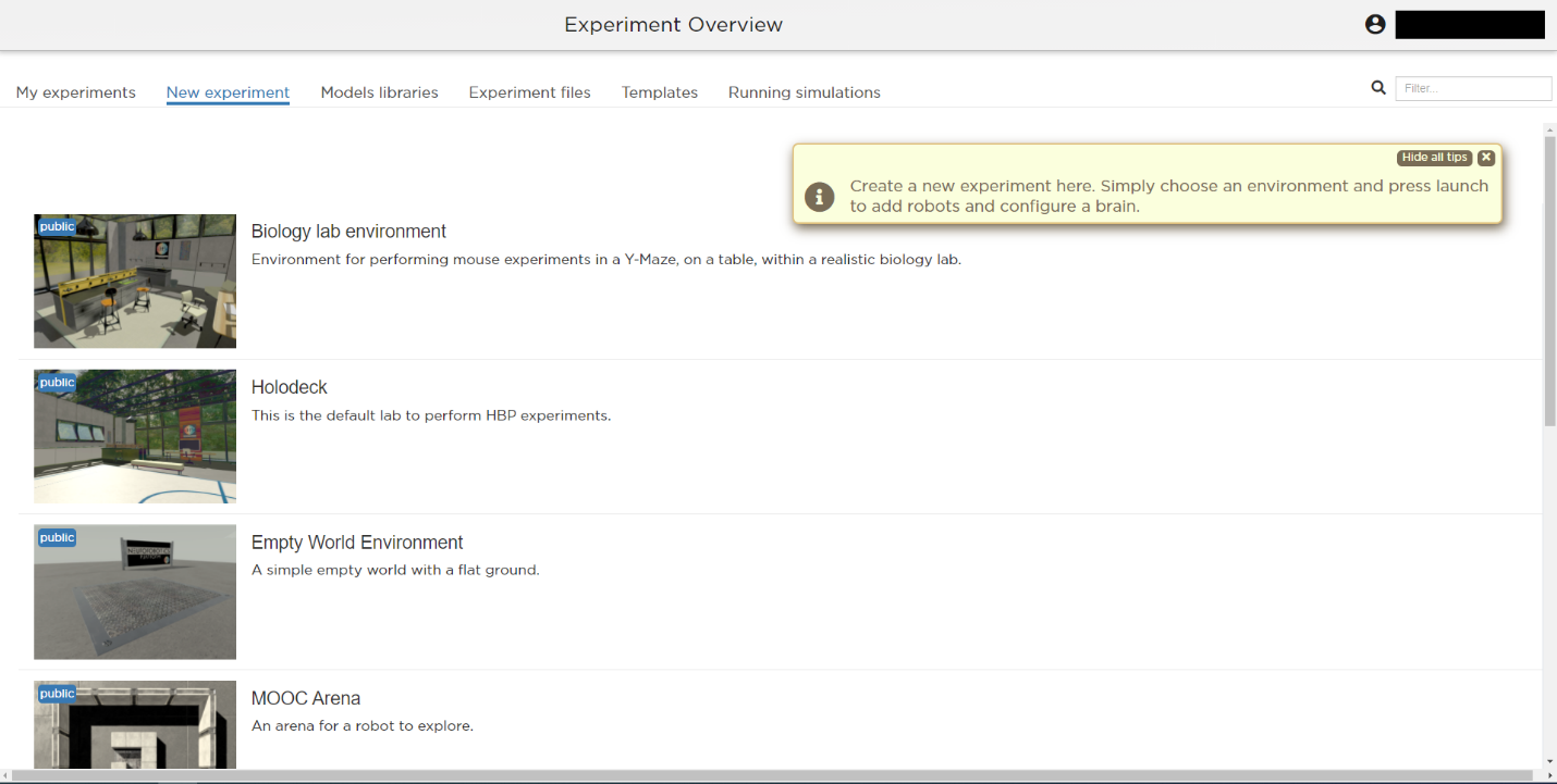
Fig. 1 The experiment overview page is the landing page of the NRP. Pop-up tips, like the one shown here, provide users with suggestions and highlight functions. You can turn these tips on and off.

In the EXPERIMENT OVERVIEW (see Fig. 1), the following multiple tabs offer different functionalities to control your simulation experience:

• My experiments: An overview of all experiments created (or cloned) by you will be displayed here.

• New experiment: A list of pre-defined, empty experimental environments. They can be selected, along with a Brain Simulator, to create a new experiment.

• Models libraries: A collection of available models organized in categories, such as environments, robots, and brains. New models may also be uploaded at your convenience to enrich your libraries.

• Experiment files: A browser-view of the files associated with user experiments.

• Templates: Experiment templates that can be cloned by all users, and subsequently run, modified, etc.

• Running simulations: An overview of all simulations that are currently running.

Detailed information on each of these tabs can be found at UI manual.

Step 2. Set up a new experiment with the tab “New experiment”

1. Click on the tab “New Experiment”

2. Click on the “Empty World Environment” list entry and select the environment. Choosing one of the available environments reveals two fields: one where the name of the experiment should be entered, and one where you can select the brain simulator of your choice.

3. From the “Brain Simulator” dropdown, select “NEST” - our choice for the example detailed in the present guide. For convenience, selecting a given brain simulator at this step automatically generates some boilerplate code inside experiment files. however, this choice can be changed later on if necessary, by modifying manually said boilerplate code.

4. Click the “Experiment Title” field and enter any name for your experiment. In this example, we’re going to name it “MyFirstExperiment”.

5. Finally, click the “Launch” button to launch the simulation.

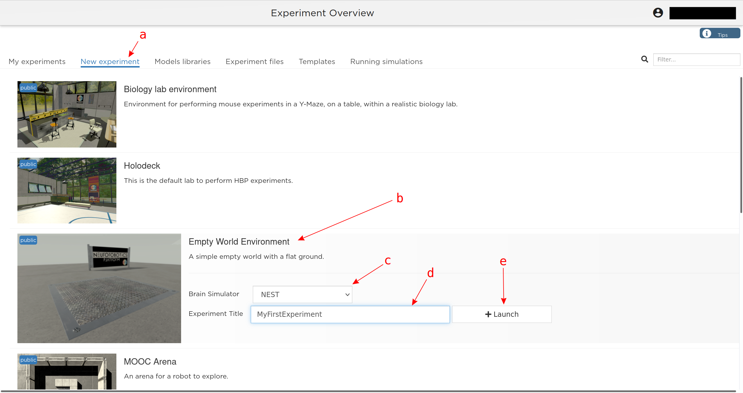
Fig. 2 Illustration of the steps to create a new experiment from a given environment.

Once the simulation is launched, a new view, referred to as the SIMULATION VIEW, is displayed (see Fig. 3). It comprises several features and functionally relevant areas. These are:

• the toolbar,

• simulation controls, and

• the display area.

The toolbar contains several entries, each yielding different color-coded functionalities to model, control, and evaluate the experiment. Green icons indicate editors, blue icons open evaluation windows, and yellow ones offer general information and help. The color-coded sections can be expanded or collapsed by clicking the small arrows at the end of each section.

Simulation controls are displayed at the top of the window. From here, one can leave, reset, start/stop the simulation, start and stop a recording, and access additional settings of the environment rendering.

The display area is where the various environment rendering, plots, consoles, etc. can be opened (through the toolbar) and arranged as per the user’s wishes and needs.

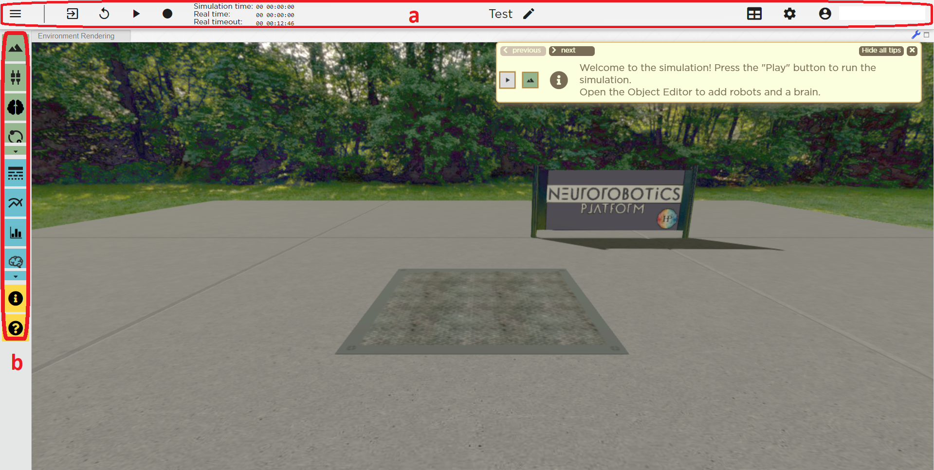
Fig. 3 Simulation view, as seen when creating a new experiment from the Empty World Environment. The two areas highlighted in red are: top, (a) - Simulation controls; left, (b) - Toolbar. The yellow window opens up at startup and shows tips.

Step 3. Add a robot to your experiment

Having created an experimental environment, you can now populate the latter with an agent. You can choose the body for this agent by searching the object library, which is located at the top of the toolbar in the simulation view and denoted by a green “mountain” icon.

The following steps, illustrated in Fig. 4, describe the procedure:

1. Click on the “Object library” in the menu bar. This will open the object library in a new tab next to the environment rendering.

2. Select “Robots” from the object categories.

3. Select any robot you wish to use. In this example, we use the “iCub HBP ros” robot.

4. Hover your mouse on the environment rendering to see the robot. Click to place it at any location.

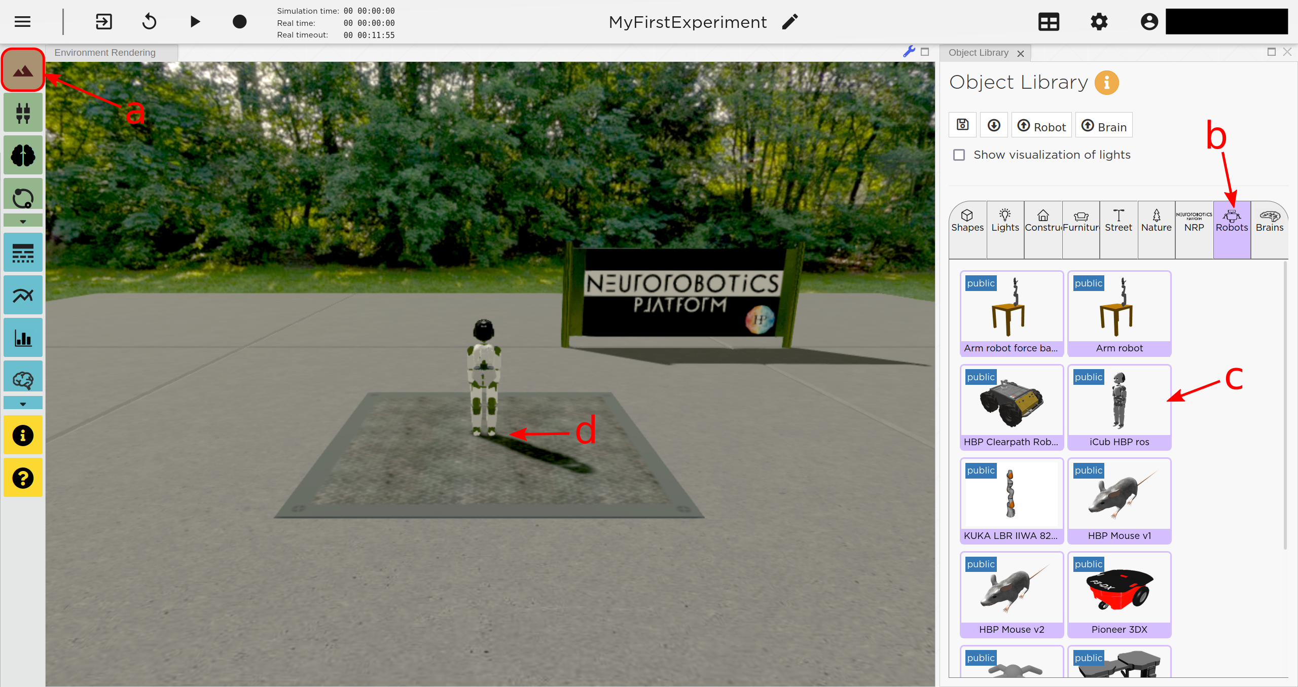
Fig. 4 Placing a robot into the environment.

Placing the robot into the environment will automatically open the OBJECT INSPECTOR. We don’t need these functionalities for now, so we may close the “Object Inspector” tab, using the little cross next to the tab’s name. It can be re-opened by right-clicking the robot and selecting “Inspect” from the context menu.

NB: You can place any object into the environment and you can even upload your own robot models into the NRP.

Note

Manipulating the camera view

You can manipulate the camera view to inspect the scene of your experiment using the keyboard or the mouse.

• Use the WASD keys or the scroll wheel to move the camera view

• Use the arrow keys or click and hold the left mouse button inside the environment rendering, then drag in the desired direction, to rotate the camera view.

By default, the view is centered on the camera itself. To center the view on any object, right-click the object, and select “Look At” from the context menu.

Step 4. Add a “brain” circuit

A fundamental step in the setting up of any experiment is the inclusion of a “brain” through the NRP BRAIN EDITOR. In most cases, it is a single neuronal circuit, the function of which we want to investigate through embodiment inside the NRP. To implement the neural circuit required in the experiment we are describing here, we use the NEST Simulator.

The NRP enables you to define a neural circuit using the PyNEST Python interface of NEST. This makes it possible to build this circuit graphically using the convenient “NEST Desktop” application, which is accessible through EBRAINS (https://ebrains.eu/service/nest-desktop/). The resulting PyNEST code can easily be transferred to the NRP.

To add a brain to the experiment, proceed as follows (illustration in Fig. 5):

1. Select the “Brain Editor” from the menu bar. It is denoted by the green icon with the brain symbol in Fig. 5).

2. Use the brain editor to implement your NEST network. You can either:

   1. import a brain script (e.g. created with NEST Desktop) using the “Upload” button

   or

   2. write your script directly in the brain editor tab.

   It’s important to note that you import the PyNEST module at the top of your script (using import nest at the top of the script).

3. Apply your changes and save them by clicking the “Apply” button.

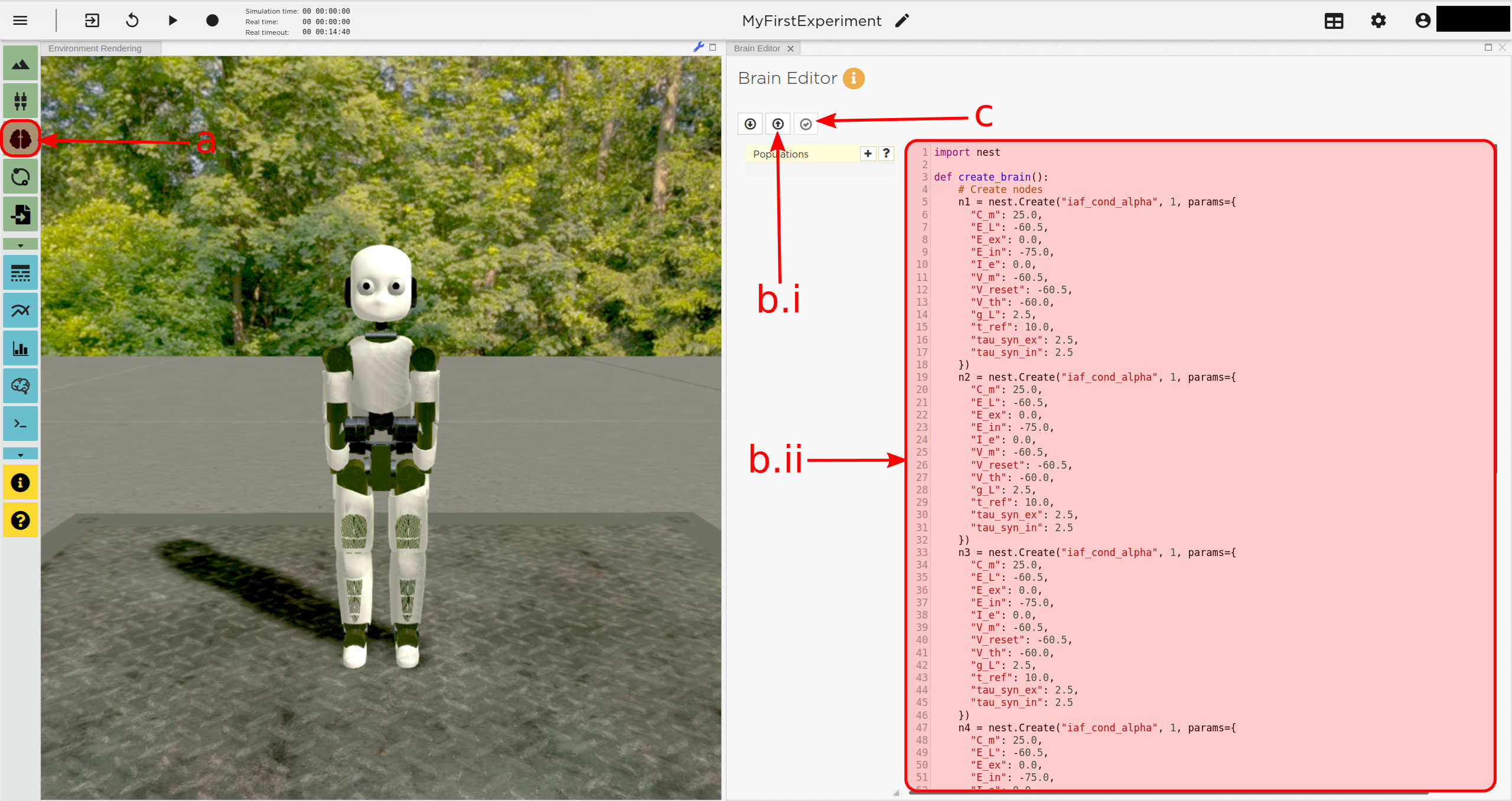
Fig. 5 Generating a brain for your robot using the brain editor.

All neuron populations that are created in the brain script will be displayed in the transfer function editor (more on that later).

Note

A little NEST trick: you can create sub-populations in the BRAIN EDITOR by slicing the “circuit” population, thus creating a more sophisticated neural architecture to be used in more complex experiments (see NEST documentation).

The brain circuit implemented in the experiment described in this guide is implemented through the following brain script, which you can copy/paste in the brain editor. Please respect the code indentation provided in the example above. In general, on the NRP, when in doubt use pythonic rules.

This script creates a network consisting of four conductance-based leaky integrate-and-fire neurons (see the reference in the NEST documentation). Two excitatory neurons connect to each other via inhibitory interneurons. Once excited sufficiently, the excitatory neurons can maintain their spiking activity through recurrent connections. Activity only stops when enough inhibitory spikes are received from the other neuron.

import nest

def create_brain():
    # Create nodes
    n1 = nest.Create("iaf_cond_alpha", 1, params={
      "C_m": 25.0,
      "E_L": -60.5,
      "E_ex": 0.0,
      "E_in": -75.0,
      "I_e": 0.0,
      "V_m": -60.5,
      "V_reset": -60.5,
      "V_th": -60.0,
      "g_L": 2.5,
      "t_ref": 10.0,
      "tau_syn_ex": 2.5,
      "tau_syn_in": 2.5
    })

    n2 = nest.Create("iaf_cond_alpha", 1, params={
      "C_m": 25.0,
      "E_L": -60.5,
      "E_ex": 0.0,
      "E_in": -75.0,
      "I_e": 0.0,
      "V_m": -60.5,
      "V_reset": -60.5,
      "V_th": -60.0,
      "g_L": 2.5,
      "t_ref": 10.0,
      "tau_syn_ex": 2.5,
      "tau_syn_in": 2.5
    })

    n3 = nest.Create("iaf_cond_alpha", 1, params={
      "C_m": 25.0,
      "E_L": -60.5,
      "E_ex": 0.0,
      "E_in": -75.0,
      "I_e": 0.0,
      "V_m": -60.5,
      "V_reset": -60.5,
      "V_th": -60.0,
      "g_L": 2.5,
      "t_ref": 10.0,
      "tau_syn_ex": 2.5,
      "tau_syn_in": 2.5
    })

    n4 = nest.Create("iaf_cond_alpha", 1, params={
      "C_m": 25.0,
      "E_L": -60.5,
      "E_ex": 0.0,
      "E_in": -75.0,
      "I_e": 0.0,
      "V_m": -60.5,
      "V_reset": -60.5,
      "V_th": -60.0,
      "g_L": 2.5,
      "t_ref": 10.0,
      "tau_syn_ex": 2.5,
      "tau_syn_in": 2.5
    })

    # Connect nodes
    nest.Connect(n1, n3, conn_spec={
      "rule": "all_to_all"
    })

    nest.Connect(n2, n4, conn_spec={
      "rule": "all_to_all"
    })

    nest.Connect(n3, n2, conn_spec={
      "rule": "all_to_all"
    }, syn_spec={
      "weight": -1.0,
      "delay": 1.0
    })

    nest.Connect(n4, n1, conn_spec={
      "rule": "all_to_all"
    }, syn_spec={
      "weight": -1.0,
      "delay": 1.0
    })

    nest.Connect(n1, n1, conn_spec={
      "rule": "all_to_all"
    }, syn_spec={
      "weight": 0.3,
      "delay": 5.0
    })

    nest.Connect(n2, n2, conn_spec={
      "rule": "all_to_all"
    }, syn_spec={
      "weight": 0.3,
      "delay": 5.0
    })

    return n1 + n2

circuit = create_brain()

Step 5. Connect body and brain with Transfer Functions

After setting up our “brain”, we now want to use it to control our robot. Therefore, the sensor outputs of the robot must be made available to the brain, and neurons have to be connected to the robot’s actuators. This can be achieved using so-called TRANSFER FUNCTIONS. For further information on Transfer Functions, see the dedicated manual.

Please note that this step involves many ROS concepts (e.g. publish/subscribe semantics, messages, topics, etc.) that it is better to be familiar with (see for example http://wiki.ros.org/ROS/Concepts).

5.1 Create a transfer function that feeds sensor data from the robot into the brain:

A transfer function (TF for brevity) is, first and foremost, a python function. As such, all pythonic concepts and quirks (decorators, indentation, etc.) apply to TFs. First, let’s create a transfer function that feeds sensor data from the robot into the brain (Fig. 6):

1. Open the “Transfer Function Editor” found in the menu bar as the green button with the “plugs” icon. In this editor, the populations defined in the BRAIN EDITOR are displayed in the “Populations” list.

2. Create a new transfer function by either

   1. Uploading a transfer function by clicking the “Upload” button

   or

   2. Creating a new transfer function using the “Create New TF” button (the large “plus”-shaped button on the top line of the Transfer Function Editor). This will create some boilerplate code that you can later edit directly inside the transfer function editor.

4. Give it a meaningful name: for instance, here, we will call it “sense”. To do so, click the default name “transferFunction” in the Transfer Function list, type in the new name, and click on the green checkmark on the same line.

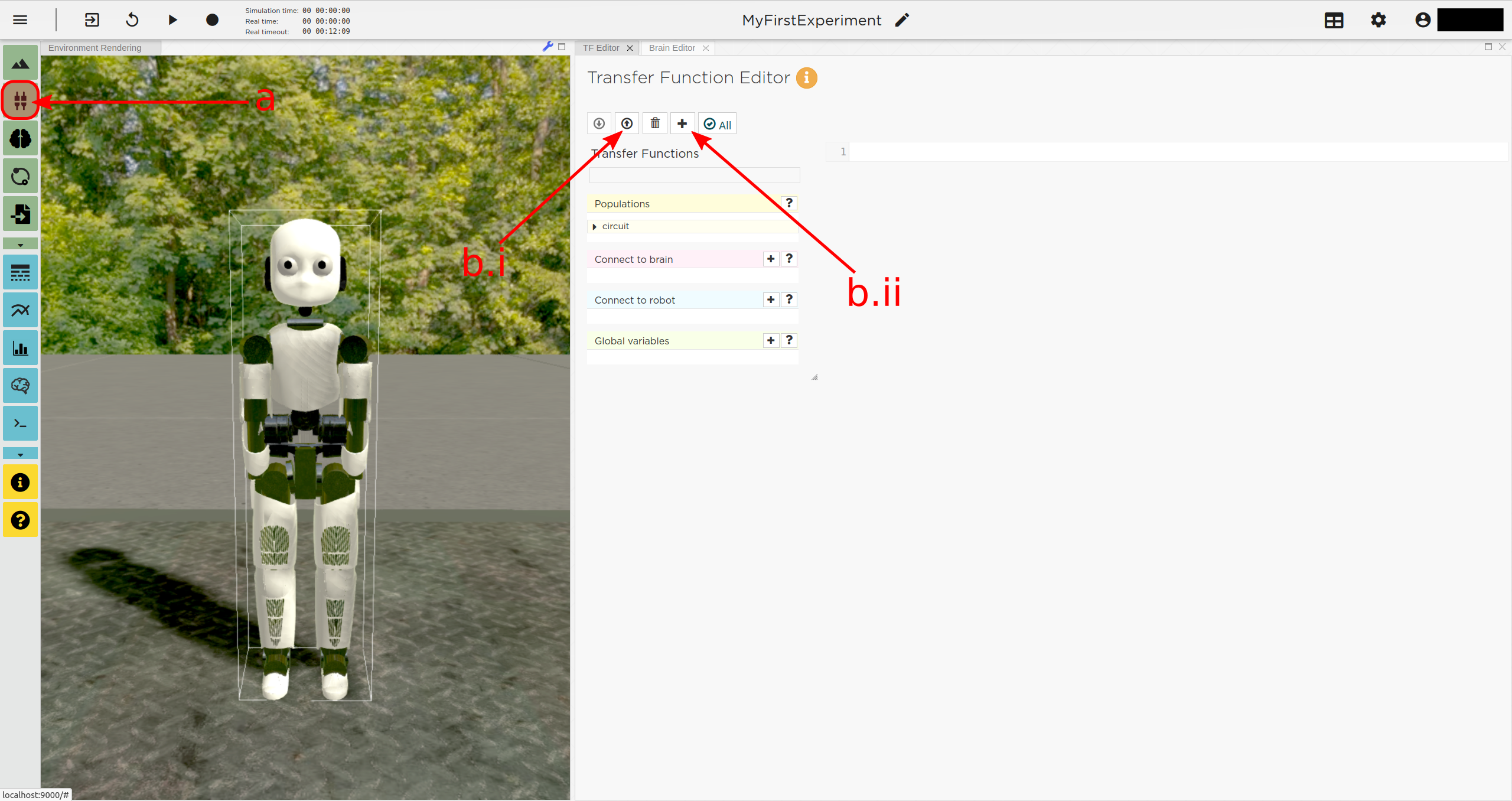
Fig. 6 Creating a new transfer function using the Transfer Function Editor

In this guide, we follow option b.ii. and create a new transfer function that we call “sense” using the “Create New FT” button.

The boilerplate code that appears in the editor upon creation of the Transfer Function uses a decorator to define the type of transfer function, namely @nrp.Robot2Neuron(). This decorator is used to define functions that feed data from the robot to the brain.

The function’s first argument is the simulation time step (which must always be the first argument of any transfer function). When created through the process followed above, the function body automatically consists of the logging of the time step, if a certain condition is met, with the clientLogger object used to write the actual messages to the log console (more on that later).

5.2 mapping a robot subscriber to a function argument

Now we map a ROBOT SUBSCRIBER to a function argument, i.e., we read a value that is being published by the robot, to make sensor data available inside our function:

1. Press the button with the “+”-sign next to the “Connect to robot” section. This will open a list of available topics to subscribe or publish to.

2. Select the topic you wish to subscribe to by clicking once on it (and highlighting it as a result). In this case, we are going to use the “/icub_hbp_ros_0/joints” topic.

3. Scroll all the way down and click the “Add Subscriber” button to confirm your choice.

   The topic is now displayed in the “Connect to robot” section and a decorator - @nrp.MapRobotSubscriber() is added to the code along with an argument to the transfer function. NB: You may also add the subscriber by typing this decorator and the function argument directly into the editor.

4. Give the topic a meaningful name - here we call it “joints” - by

   1. expanding the topic (by clicking on it) in the “Connect to robot” section and editing the corresponding field,

   2. or by changing it directly in the decorator using the editor. NB: doing so in the decorator also requires manually changing the function argument to match the new name of the topic.

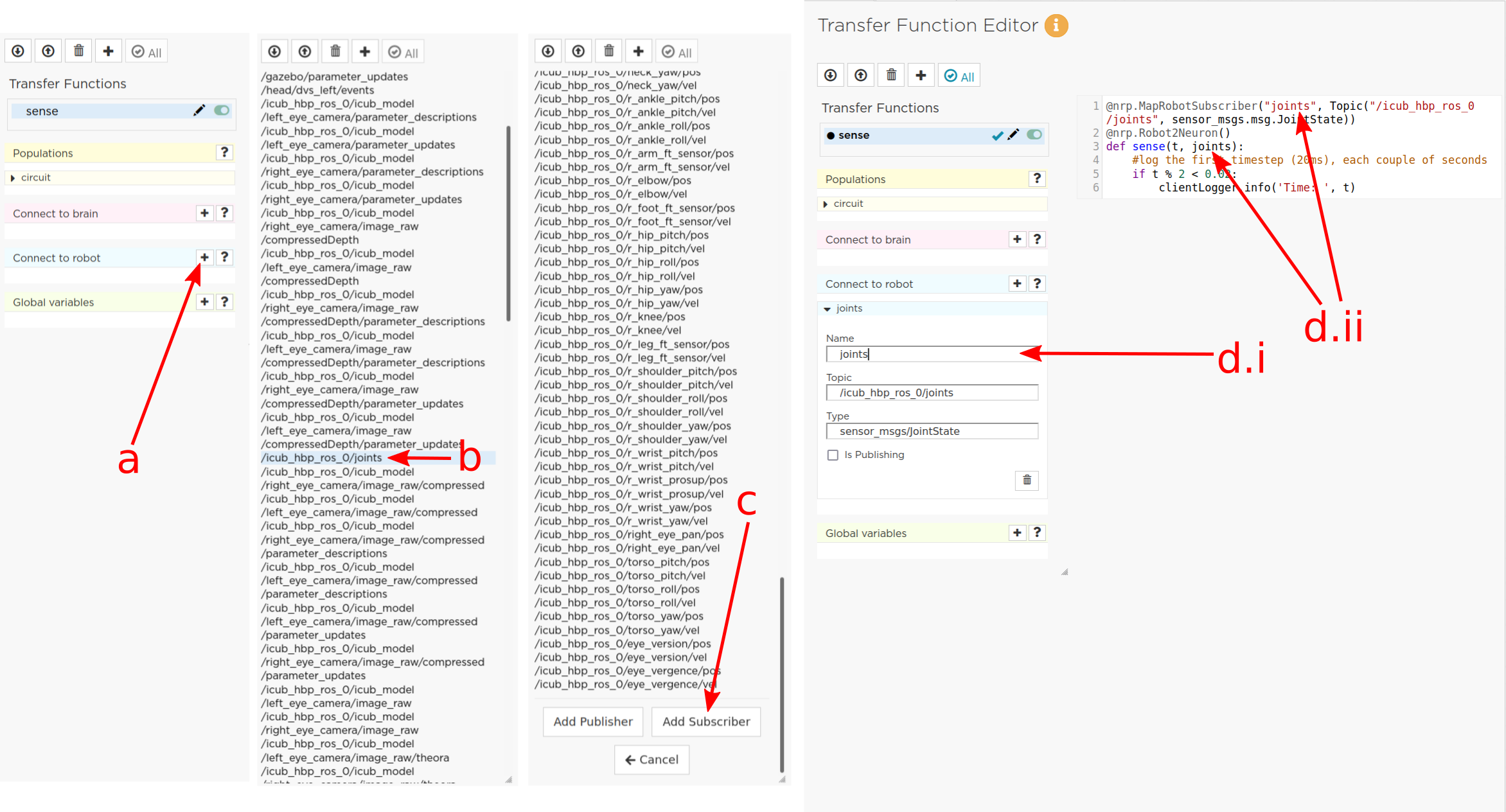
Fig. 7 Adding a robot subscriber to the transfer function.

5.3 Perform some basic testing

Now that we have set our sensor input, let us perform a simple but essential check that everything works as expected, and let us take a look at the contents of the messages published by the sensor. For this purpose, you will log these contents to the “Log Console” from within a transfer function using the clientLogger object. Please note that the latter doesn’t have to be imported nor created; it is already available in the scope of the function.

1. Include the following line in the template function body to log our new message in the console:

   clientLogger.info(joints)
   

   This line will write a timestamp along with the contents of the argument (in this case: the variable “joints”) into the Log Console at every time step. NB: Pay attention to pythonic indentation rules!

2. Press the button designated by the red arrow in Fig. 8 to open this Log Console - note that, depending on the size of your screen, you may have to expand the blue section of the toolbar to find this button. We can now apply the changes to the transfer function (green checkmark near the TF name) and start the simulation via the play button in the “Simulation Control” bar at the top of the window.

3. See and verify that the “joints” variable holds an object of type “RosSubscribedTopic”.

4. Change the clientLogger.info(joints) line to the following in order to log the actual message contents:

   clientLogger.info(joints.value)
   

After applying the changes to the transfer function (green checkmark sign), you should now see the message contents. The message contains some meta-data, a list of joint names, and three arrays containing position, velocity, and effort values.

You can pause the simulation to inspect the console outputs by pressing the large “pause” button in the “Simulation controls” (see Fig. 3).

When testing the experimental setup, it is often useful to check that some values correspond to expectations for which we possess a high degree of confidence. Let us suppose that, for this purpose, we want to retrieve the position of the roll-axis of the left shoulder, as we are confident about the range they should be in. To do so, delete the logging command and insert the following lines of code into the function body:

l_shoulder_roll = joints.value.position[joints.value.name.index("l_shoulder_roll")]
clientLogger.info("Left shoulder roll: {}".format(l_shoulder_roll))

The first line retrieves the position of the left shoulder roll axis from the “position” array of the message. It, therefore, uses the index of the “l_shoulder_roll” value in the “name” list, and stores it into the variable l_shoulder_roll. The second line logs this value into the console. Upon restarting the simulation, the values should appear in the console, as expected. You are all set to go to the next step!

Note

The names of topics, the message types, and structures are specific to the robot model. They will be different from other robot models.

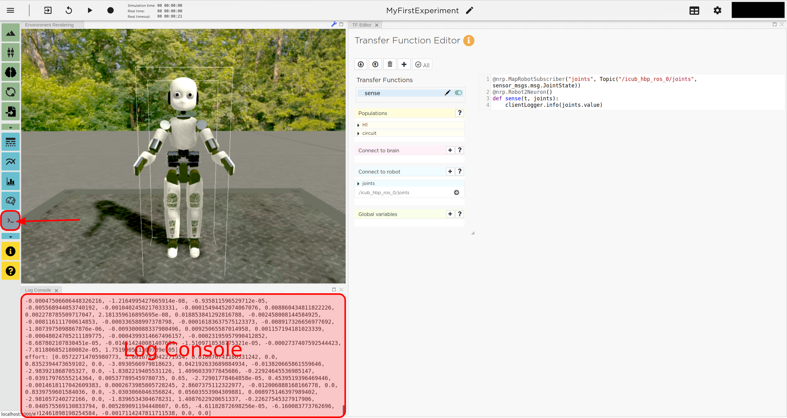
Fig. 8 Opening the “Log Console”.

5.4 Create a device to drive brain activity with sensor output:

Gazebo (our robotic simulation) can now send sensor data to our “brain” that is implemented inside the NEST simulator. In the next sections, you will learn how to handle this data so that NEST can make sense of it via so-called “devices”, which are the software constructs that allow us to establish such a connection between NEST and the rest of the NRP.

Concretely, in the following, we will create such devices and will define thresholds for sensor signals as input that, when crossed, trigger the devices to send spikes to neurons into the NEST “brain”.

To create a device, follow the instructions below and refer to Fig. 9:

1. Click the “+” sign next to the “Connect to brain” section in the Transfer Function Editor. The available neuron populations are displayed.

2. Click on the right-facing black triangle close to the name “circuit” to expand the “circuit” population. This reveals two neurons. Select the first neuron.

3. Click the “Create Device” button.

4. Rename the device (click on its name to edit it). Here, we will call it “lower_threshold”.

5. Select “Poisson Generator” in the “Type” dropdown-list of the device.

6. Create a second device, connected to the second neuron, by repeating steps a-e, and name this device “upper_threshold”.

7. Click the green tick mark that sits beside the name of the TF (“sense”) to make sure that the changes are saved.

We have now created two Poisson generators, that are connected to our brain circuit.

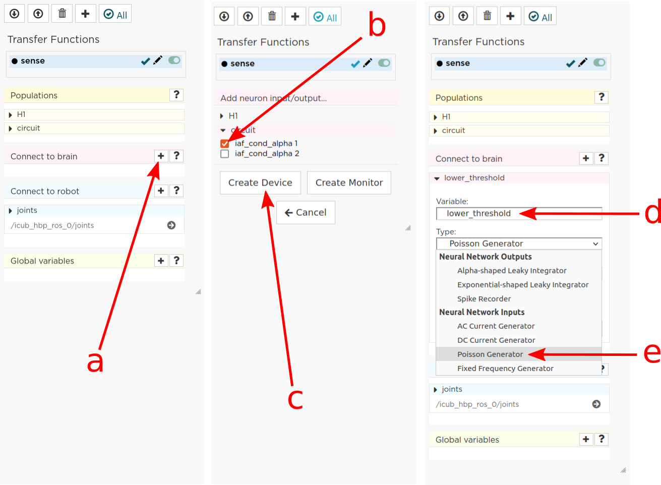
Fig. 9 Adding a device to feed sensor data into a neuron in NEST.

5.5 Configuring the Poisson generators

Now, paste the lines in the box below at the end of the body of the “sense” transfer function, in the text editor. As usual, pay attention to indentation.

lower_threshold.rate = 500. if l_shoulder_roll < 1.8 else 0.
upper_threshold.rate = 500. if l_shoulder_roll > 2.4 else 0.

These lines set the rates of the Poisson generators depending on the current position of the robot left shoulder.

Our excitatory neurons are now receiving excitatory signals in the shape of Poisson spike trains whenever the left shoulders roll-axis position takes values above or below the specified threshold values of 1.8 and 2.4.

Step 6. Close the loop: connect the brain to the body

In the previous section, we have connected the sensor outputs of the robot to the brain. The next step is to connect the brain to the robot’s actuators. This will allow us to control the robot’s movements using the brain’s activity.

To do this, we create another transfer function, this time mapping neuron activity to the robot. The following steps along with Fig. 10 describe how to achieve this.

1. Add a new transfer function in the Transfer Function Editor (use the “Create new TF” button illustrated in Fig. 6, as described in section 5.1). We will call it “act”.

2. Change the decorator of the template function from

   @nrp.Robot2Neuron()
   

   to

   @nrp.Neuron2Robot(Topic("icub_hbp_ros_0/l_shoulder_roll/vel", std_msgs.msg.Float64))
   

   This decorator maps the return value of the function to the specified topic.

3. Add two devices in the “Connect to brain” section (see section 5.4), each connecting to one of the neurons in our circuit. We will name the device connecting to the first neuron “up_motion”, and the other one “down_motion”. Set their type to “Alpha-shaped Leaky Integrator”. The mathematical details behind the function of these devices are beyond the scope of this guide and can be found elsewhere (e.g. https://neuronaldynamics.epfl.ch/online/Ch1.S3.html). Note that these steps add decorators above the body of the “act” TF.

4. In the editor, insert the following line in the body of the “act” TF, replacing the template code:

   return 1.0 + 10.0 * (up_motion.voltage - down_motion.voltage)
   

   This line computes the value we want to set as the left shoulder roll axis velocity and returns it. We are using 1.0 as our resting value. The voltage values of the leaky integrators are scaled by a value of 10.0 and added to the resting value.

5. Apply the changes to the transfer function (green tick mark to the right of the TF name).

6. Restart the simulation (“play” button on the Simulation Controls).

The robot should now start waving its left arm!

Note

The simulation can get stuck in states that are undesirable, especially if the scripts are changed on the fly. If that happens, it may help to stop and leave the simulation, and then relaunch it.

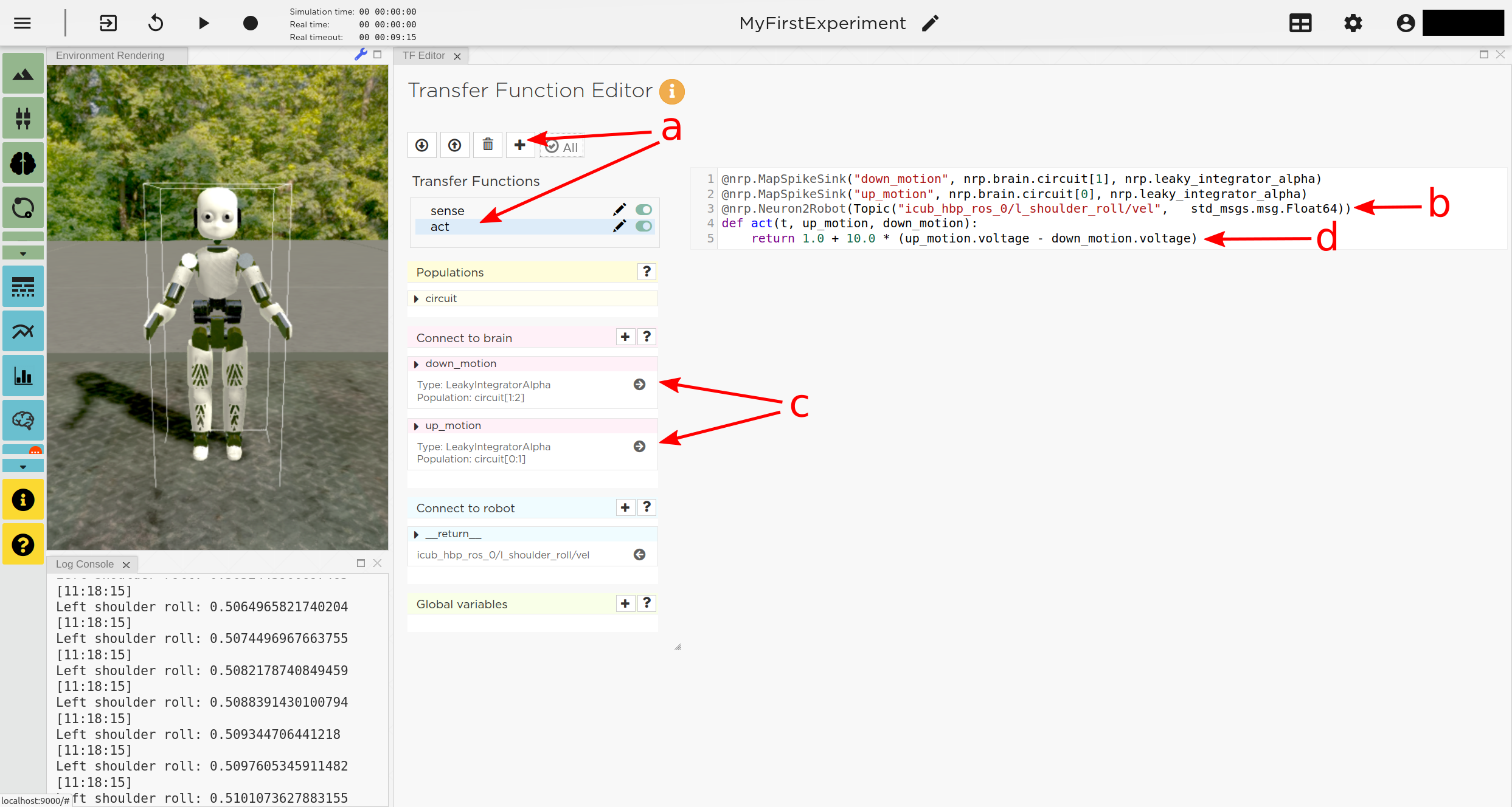
Fig. 10 Adding a transfer function connecting the brain activity to the robot’s actuator.

Step 7. Monitor neuronal activity during the simulation with the ‘Spiketrain Monitor’

After setting up all functional parts of the experiment, we might want to observe the underlying neuronal activity, therefore we are going to add a so-called NEURON MONITOR.

The following steps (illustrated in Fig. 11) show how to add a neuron monitor and observe the activity using the “Spiketrain” monitor tool.

1. Open the Menu Bar, select and launch the “Spiketrain” Monitor.

2. In the Transfer Function Editor, select any transfer function (its exact identity does not matter: see step d) and click the “+” sign next to the “Connect to brain” section.

3. In the “Add neuron input/output…” menu, select all neurons of the circuit.

4. Click the “Create Monitor” button. A new transfer function will be added automatically.

5. Set the type of the device to “Spike Recorder”.

6. Apply changes to the new monitor TF (green tick mark to the right of the TF name).

7. Start the simulation (“play” button on the Simulation Controls). The spike trains should now be displayed in the “Spike Train” tab.

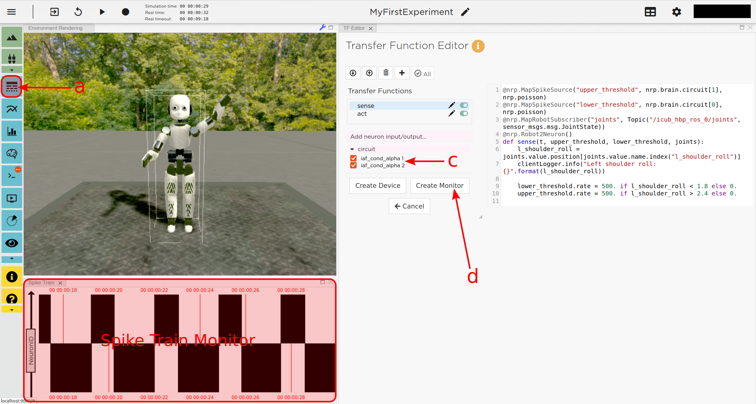
Fig. 11 Adding a Spike Train Monitor.

Step 8. Postprocessing: record data into CSV files.

Data from the experiments can be recorded into files for postprocessing. The TF framework offers mechanisms to store data in the CSV format.

To create a Transfer Function that records spikes into a CSV file you need to

1. Create a new Transfer Function in the Transfer Function Editor and name it “csv_spike_monitor”.

2. Add a new device in the “Connect to brain” section, connecting to all neurons in the circuit. Set its name as “spikes” and its type to “Spike Recorder”. One can now inspect the contents of this device by using

   clientLogger.info(spikes.times)
   

   in the function body. The “times” field of the “SpikeRecorder” object holds a list of spikes. Each spike is itself a list, with the first entry representing the neuron’s identifier, and the second entry the spike’s timestamp.

3. Add a new variable and name it “recorder” in the section “Global variables” (as before, use “plus” sign to add the variable).

4. Set up the recorder as follows:

   1. Select “CSV Recorder” as its type.

   2. Give a file name. In this case: “all_spikes.csv”.

   3. Add headers by writing a name into the “Header” field and pressing the “+” button to submit. In this guide, two headers - namely “ID” and “TIME” - are used.

5. Insert this piece of code into the function body:

   for entry in range(len(spikes.times)):
      recorder.record_entry(
            spikes.times[entry][0],
            spikes.times[entry][1]
      )
   

The first line defines a loop over all elements of the list in the “times” field. The remaining code uses the “record_entry” method of the CSVRecorder object stored in the “recorder” to write each spike into the CSV file. Note that the order of the input arguments to the “record_entry” method should match the order in which the headers were defined during step d.iii.

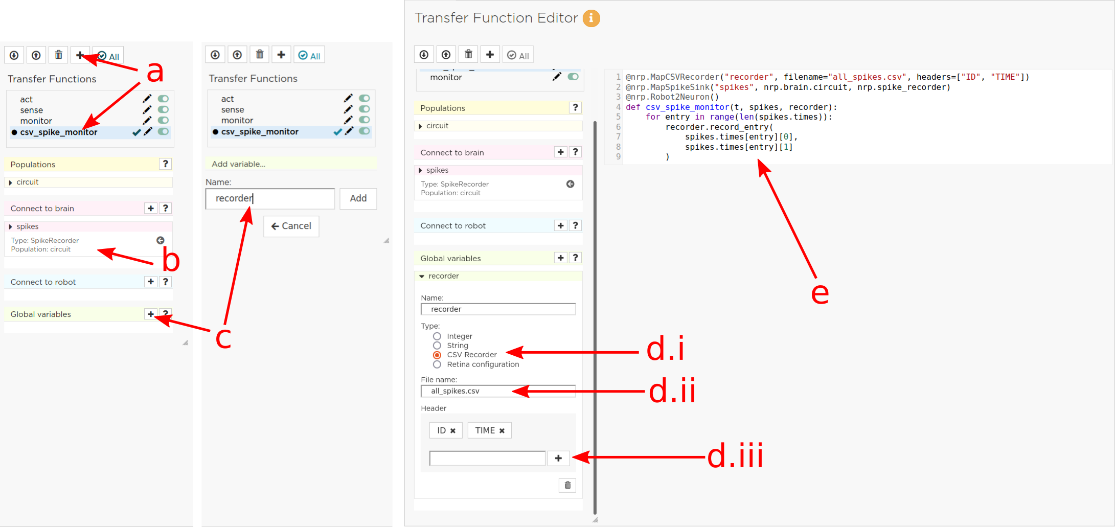
Fig. 12 Create a Transfer Function to record experiment data into a CSV file.

If you wish to add another recorder for the left shoulder roll position of the robot, repeat steps a-d with the following modifications:

1. Name the Transfer Function “csv_joint_monitor”.

2. Add a subscriber in the “Connect to robot” section that subscribes to the “/icub_hbp_ros_0/joints” topic and name it “joints” (see section 5.2).

3. Add a new variable and name it “recorder” in the section “Global variables”.

4. Set up the recorder as before, but make sure to use a different file name, e.g. “l_shoulder_roll.csv”. As for the headers, name them “TIME” and “POS”.

5. Insert the following piece of code into the function body:

   l_shoulder_roll = joints.value.position[joints.value.name.index("l_shoulder_roll")]
   recorder.record_entry(t, l_shoulder_roll)
   

The first line reads the position of the joint, as in the “sense” Transfer Function. The remaining code again stores the values using the “record_entry” method. This time, the default Transfer Function argument “t”, representing the simulation time, is stored alongside the joint position.

6. Apply all changes (green tick mark to the right of the TF name) and run the simulation. At this point, the CSV files can be found in the “Experiment files” tab of the “Experiment overview”. The files can be downloaded and used for further processing.